LLM Metacognition: Shared and Shallow?

M. Moran

Mar 31, 2026

Across 19 frontier models, metacognitive confidence on question and answer tasks tracks a shared difficulty heuristic with only a weak relationship to actual performance.

‍

Do models know what they don't know? Asking a model to predict whether it can answer a question before attempting it is already standard practice in agentic systems. Models are better than chance at it. But where does that signal come from? We're testing 19 frontier models across multiple benchmarks using psychometric methods borrowed from outside ML, and so far what we've found is shared and shallow: models converge on similar confidence behaviors regardless of actual ability, suggesting a heuristic absorbed from training data rather than genuine self-knowledge. To confirm, we used a steering vector to directly manipulate metacognitive assessments and matched each model's behavior to the others.

Setting the task

We started with SQuAD, an information extraction benchmark where a model receives a question and a relevant Wikipedia passage and extracts the answer. It's been saturated since 2019, so we removed the passage and kept only the question, converting it into a closed-book recall task on data the models were almost certainly trained on. Modifying an older benchmark keeps us squarely in distribution while remaining an unlikely target for explicit calibration. If a model can't reliably assess whether it can recall facts from its own training data, that's a poor sign for its ability to predict performance on complex agentic workflows.

On top of this recall task we layered a metacognitive one. Each model is presented with a question and asked "do you think you can answer this correctly?", giving its reasoning before answering yes or no. We treat that yes or no as the output of a binary classifier and check how well it matches actual performance.

Figure 1. Metacognitive F-beta score as a function of risk attitude across all 19 models. Low beta (left) penalizes overconfidence. High beta (right) penalizes underconfidence. No single model dominates across the full range, and the best model changes depending on what kind of error is most impactful.

‍

F1 scores cluster between 0.6 and 0.8 across models. To break the symmetry on false positives and false negatives, we extended to F-beta, which generalizes F1 by weighting precision against recall: low beta penalizes overconfidence, high beta penalizes underconfidence. No single model dominates the full range. Claude was cautious, GPT was eager. Which end of the sweep you want depends on your deployment: sometimes a wrong answer is catastrophic, sometimes it costs nothing.

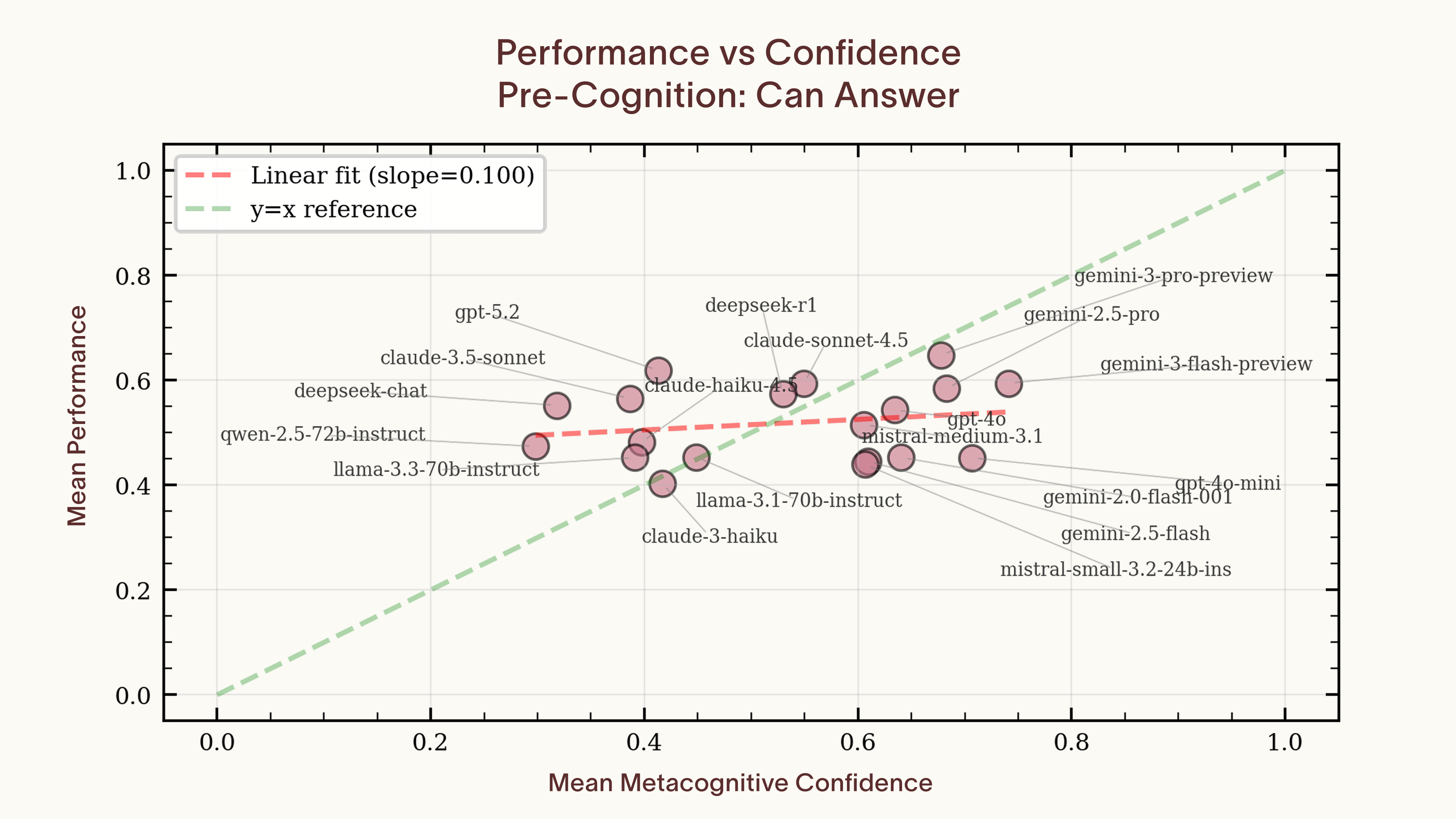
Figure 2. Average performance vs. average confidence across 19 frontier models on SQuAD. The dashed green line is perfect calibration (y = x). The red fit line (slope = 0.097) shows that confidence and actual accuracy on a between-model basis are nearly unrelated.

‍

The per-question F1 scores look reasonable. The cross-model picture is harder to explain. We plotted each model's average confidence against its average accuracy and found no significant correlation (slope = 0.097, p = 0.5). Individual models are well-calibrated in aggregate, but confidence doesn't track ability across models. To understand what's driving that gap, we need to move past the aggregate statistics and look at the question-by-question structure.

One signal, nineteen thresholds

We started with the most deflationary explanation: models are pattern-matching surface cues from shared training data. Only if we failed to reject that would we need to invoke anything richer. A falsifiable prediction of this hypothesis is that the variance in metacognitive predictions across models should have a low-dimensional structure. Our first thought was to do PCA on the data and report the effective dimensionality that way, but PCA doesn't work on binary data and invents phantom dimensions.

We turned instead to tetrachoric correlation, a technique from psychometrics designed for exactly this situation.

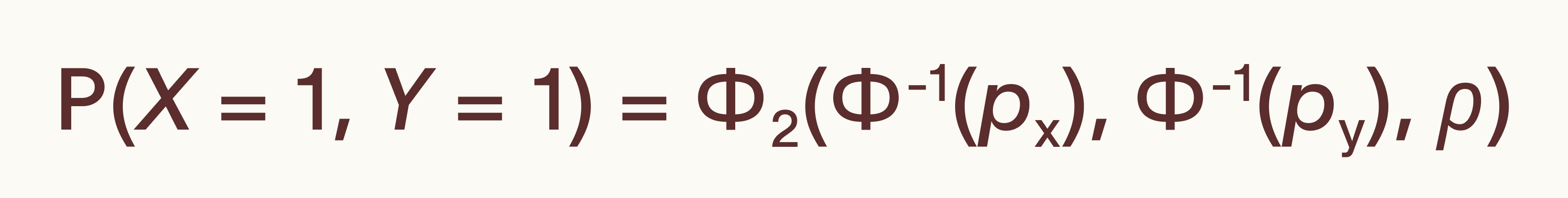
Equation 1. The formal stuff: Tetrachoric correlation assumes each pair of binary responses originates from a thresholded bivariate normal. Φ₂ is the bivariate normal CDF, pₓ and pᵧ are the marginal yes-rates of models X and Y, Φ⁻¹ maps these to thresholds on the latent normal scale, and ρ is the latent correlation we wish to recover. Fitting ρ for every pair of models gives us a correlation matrix in the assumed continuous space, which can then be analyzed like any other continuous correlation matrix. Each pair is evaluated in isolation so the assumption is self-testing. If the combined space is inconsistent and the assumptions are false, then you get strong negative eigenvalues when you attempt PCA.

‍

The assumption here is that binary observations are just a thresholding of an underlying continuous process, which produces noisier binary splits close to the boundary. For LLMs this is barely an approximation: the binary response is a thresholding of continuously computed logits. Fitting the tetrachoric correlation for every pair of models gives us a correlation matrix from the underlying continuous space. If our assumption is false, the correlation matrix will be self-inconsistent and the analysis will fail. On this matrix we can derive a latent factor space. One factor per model.

The latent factor space gives each question a score on every extracted dimension, and each model two numbers per dimension: a loading, which captures how strongly that dimension correlates with its responses, and a threshold, which is the cutoff on the latent difficulty scale above which it says no, derived from each model's marginal yes-rate. A loading near 1 means the dimension almost fully determines the model's responses. A loading near 0 means it's ignoring that dimension entirely. Two models can have identical loadings, picking up on exactly the same signal, but set different thresholds, so one says yes where the other says no. If one dimension explains most of the variance, the whole space collapses to a single shared difficulty scale: every model is reading the same cues from the question, and the only thing that differs is how cautious it is. If multiple dimensions survive, different models are picking up on genuinely different things.

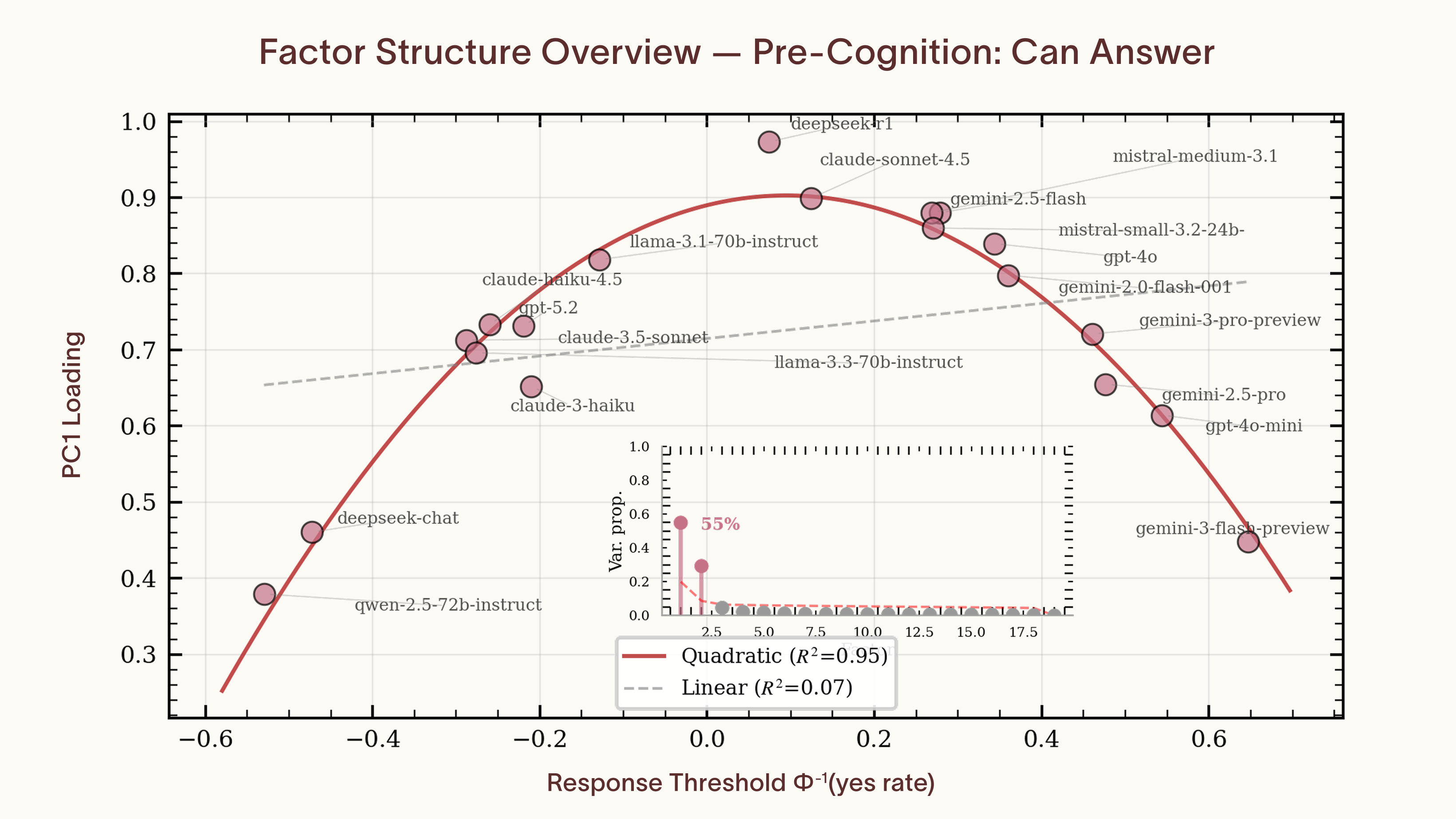
Figure 3. Factor structure overview. The main plot shows each model’s loading on the first factor (y-axis) against the corresponding response threshold (x-axis). The inset shows the variance explained by each factor, with the first accounting for 55% and the rest near the noise floor computed from permuting the binary response matrix. The quadratic fit (R² = 0.95) confirms that the apparent second dimension is driven by threshold effects at the extremes and simply encodes the models base yes / no rates rather than real structure. The same phantom structure is present on the null distribution, which has a single dominant eigenvalue explaining ~2% of the permuted distribution variance.

‍

The structure of the metacognition we found is trivial. Models share a common model of question difficulty and each picks an arbitrary cutoff for saying no. Tetrachoric correlations leave room for an independent factor per model, yet a shared estimated difficulty factor explains 55% of the variance between models. Models near the center of the yes-rate distribution load above 0.9 on the shared factor, while those at the extremes drop off along a quadratic curve (R² = 0.95).

The second factor, which accounts for 30% of the variance, is a known artifact of tetrachoric analysis. Models at the extremes of the threshold distribution end up with nearly all-yes or all-no response patterns except on trivially easy questions or ones that are impossible to parse. With so few meaningful disagreements, the tetrachoric estimate for those models becomes noisy. That noise depresses their loading on the true shared factor, and the residual variance lands in a second component that tracks yes-rate rather than anything about the questions themselves.

We confirmed this with permutation nulls. For each null, we preserved every model's yes-rate but scrambled question identity, destroying any shared signal while keeping the marginal statistics intact. The null distributions produce a second factor at roughly 25% with the same relative loadings as the one in our real data. The second factor in our real data is statistically identical to the one produced when there is no shared structure to find. Filtering it out, the data is one-dimensional up to the noise floor. Each question has a position on a shared difficulty dimension, and each model has a threshold on that dimension: questions below the threshold get a yes, questions above it get a no. The models aren't assessing their own abilities. They're just sitting at different points on the same scale.

Operationalizing the insight

The shared signal probably isn't self-knowledge. Genuine self-knowledge would be model-specific. Similar post-training regimes, representational convergence at scale, and overlapping training data could each produce this shared factor, and these explanations aren't mutually exclusive. But regardless of which shallow mechanism dominates, the shared factor is directly testable. If we can locate a direction in one model's activation space, steer along it, and reproduce another model's confidence patterns, that is evidence the factor is real.

We used Mistral-7B for the steering experiment, choosing a model outside the original set specifically because it's out of distribution. We computed steering vectors by presenting the metacognitive questions and extracting the mean activation vector between yes and no responses. For each of the 19 target models, we found the steering magnitude that caused Mistral-7B to best match that model's yes/no behavior.

Figure 4. Each target model’s factor threshold (x-axis) vs. the Mistral-7B steering magnitude that best reproduces its confidence behavior (y-axis). The near-linear relationship confirms that a single parameter, applied to one model, is enough to reconstruct any other model’s yes/no pattern.

The optimal steering magnitude tracks each model's threshold on the shared difficulty factor (R² = 0.78). One scalar, applied to one model, reconstructs the confidence profile of any model in the set to roughly 80% agreement, with an R² of 0.78 on the optimal steering coefficient as a function of the difficulty threshold on the shared factor.. The shared factor isn't an artifact of how we analyzed the data. It corresponds to a concrete direction in activation space, and varying the magnitude along that direction moves a model's confidence threshold to match any of the original 19.

This has immediate practical use. The shared difficulty heuristic is imperfect, but it outperforms random prediction of whether a model will answer correctly, and the steering vector gives you direct control over it. Rather than sampling multiple models to estimate the question's shared difficulty factor, you can adjust the threshold on the single model you're running. If you want to cut the LLM out of confidence gating entirely, a small classifier trained on the inferred difficulty labels would likely match its performance at a fraction of the cost. If you prefer an external harness, these results tell you the signal it would need to replicate is one-dimensional and model-agnostic.

Where this leaves us

Do models know what they don't know? They report what they know with reasonable accuracy, but what they report tracks a shared difficulty heuristic, not their individual capabilities. The confidence structure is simple enough that a steering vector or LoRA can shift the threshold. But the heuristic works on obvious cases where all models are interchangeable and breaks down where it would matter most: out-of-distribution, high-stakes scenarios. Otherwise we'd see a stronger cross-model correlation between confidence and accuracy. An F1 of 0.7 is an F1 of 0.7, and you can shift the threshold to match your risk tolerance. Just don't expect it to generalize. Running multiple models won't help either. They're all using the same mechanism.

A confidence signal that works on in-distribution cases and fails on out-of-distribution ones isn't just imperfect. It's a trap. It passes validation precisely where you didn't need it and fails silently where you did. Verbalized confidence is the most widely deployed gating mechanism in production systems that can't directly verify answers, and it mostly tracks a shared difficulty heuristic rather than actual competence. Either we find ways to induce genuine self-introspection, or we stop asking the model and verify externally.

This work left us with more questions than answers. Does the finding generalize beyond fact recall to coding or mathematical reasoning? If we control for the shared factor, is there anything in the residuals that tetrachoric analysis missed, or is it noise? We will publish further analysis shortly. What's certain is that F1 scores alone don't capture what's happening here, and that the apparent simplicity of self-assessment is precisely what limits its usefulness at the hard-to-verify frontier of model capabilities.

‍

This study was led by M. Moran, with contributions from @MarkWhiting and @phoebeyao, and originates from our team at @hellopareto.